Compute and Plot Correlation Matrix for a Set of General Circulation Models
Source:R/cor_gcms.R
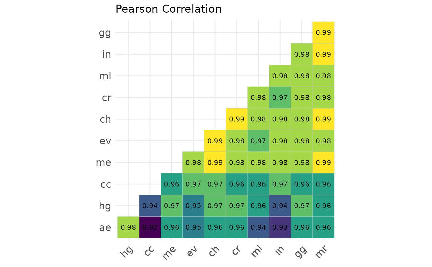
cor_gcms.RdThis function computes and visualizes the correlation matrix for a set of General Circulation Models (GCMs) based on their variables.
Usage
cor_gcms(
  s,
  var_names = c("bio_1", "bio_12"),
  study_area = NULL,
  scale = TRUE,
  method = "pearson"
)
Arguments
- s
A list of stacks of General Circulation Models (GCMs).
- var_names
Character. A vector with names of the variables to compare, or 'all' to include all variables.
- study_area
An Extent object, or any object from which an Extent object can be extracted. Defines the study area for cropping and masking the rasters.
- scale
Logical. Whether to apply centering and scaling to the data. Default is
TRUE.- method
Character. The correlation method to use. Default is "pearson". Possible values are: "pearson", "kendall", or "spearman".
Value
A list containing two items: cor_matrix (the calculated correlations between GCMs) and cor_plot (a plot visualizing the correlation matrix).
Examples
var_names <- c("bio_1", "bio_12")
s <- import_gcms(system.file("extdata", package = "chooseGCM"), var_names = var_names)[1:5]
study_area <- terra::ext(c(-80, -70, -50, -40)) |>
  terra::vect(crs="+proj=longlat +datum=WGS84 +no_defs")
cor_gcms(s, var_names, study_area, method = "pearson")
#> CRS from s and study_area are not identical. Reprojecting study area.
#> Scale for fill is already present.
#> Adding another scale for fill, which will replace the existing scale.
#> $cor_matrix
#>           ae        cc        ch        cr        ev
#> ae 1.0000000 0.9978482 0.9692338 0.9735887 0.9874646
#> cc 0.9978482 1.0000000 0.9632915 0.9684004 0.9804430
#> ch 0.9692338 0.9632915 1.0000000 0.9994263 0.9934712
#> cr 0.9735887 0.9684004 0.9994263 1.0000000 0.9942620
#> ev 0.9874646 0.9804430 0.9934712 0.9942620 1.0000000
#>
#> $cor_plot

#>
#>