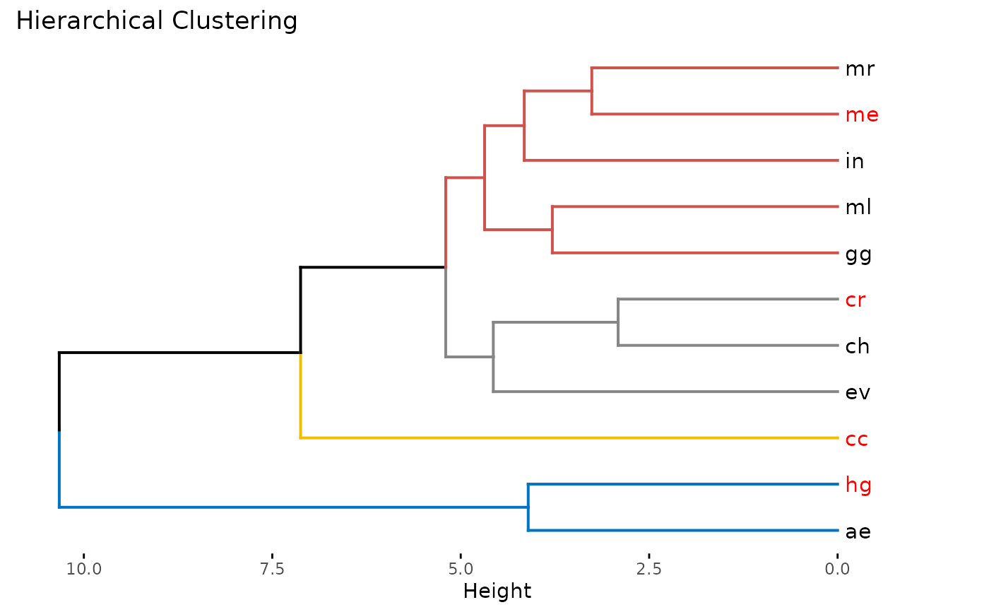
This function performs hierarchical clustering on a random subset of raster values and produces a dendrogram visualization of the clusters.
Usage
hclust_gcms(
  s,
  var_names = c("bio_1", "bio_12"),
  study_area = NULL,
  scale = TRUE,
  k = 3,
  n = NULL
)
Arguments
- s
A list of stacks of General Circulation Models (GCMs).
- var_names
Character. A vector of names of the variables to include, or 'all' to include all variables.
- study_area
An Extent object, or any object from which an Extent object can be extracted. Defines the study area for cropping and masking the rasters.
- scale
Logical. Should the data be centered and scaled? Default is
TRUE.- k
Integer. The number of clusters to identify.
- n
Integer. The number of values to use in the clustering. If
NULL(default), all data is used.
Examples
var_names <- c("bio_1", "bio_12")
s <- import_gcms(system.file("extdata", package = "chooseGCM"), var_names = var_names)[1:5]
study_area <- terra::ext(c(-80, -70, -50, -40)) |>
  terra::vect(crs="+proj=longlat +datum=WGS84 +no_defs")
hclust_gcms(s, var_names, study_area, k = 4, n = 500)
#> CRS from s and study_area are not identical. Reprojecting study area.
#> $suggested_gcms
#> [1] "ae" "cc" "cr" "ev"
#>
#> $dend_plot

#>
#>