ECDF and Mahalanobis Distance for Theoretical Niche Modeling

Introduction

This vignette shows how to use the ECDFniche package to reproduce the simulations from the original ECDF_MahalDist.R script, comparing Mahalanobis distance-based suitability transformations using the chi-squared distribution and the empirical cumulative distribution function (ECDF).

library(ECDFniche)
#> Registered S3 methods overwritten by 'ggpp':
#>   method                  from   
#>   heightDetails.titleGrob ggplot2
#>   widthDetails.titleGrob  ggplot2

Core simulation: `ecdf_theoretical_niche()`

The function ecdf_theoretical_niche() simulates a multivariate normal “environmental space”, computes Mahalanobis distances for a sample of points, and then maps those distances to suitability using:

$1 - F_{\chi^2}(D^2)$ (theoretical chi-squared transformation)
$1 - \text{ECDF}(D^2)$ (empirical transformation)

set.seed(3)
res1 <- ecdf_theoretical_niche(n = 2)
res1$corplot

The returned list contains:

corplot: correlation vs sample size between the “true” niche and both suitability transformations
sample_data: matrix with the last sample of environmental predictors
sample_niche, chisq_suits, ecdf_suits: suitability values
mahal_dists: Mahalanobis distances for the last sample

You can directly plot the correlation object:

res1$corplot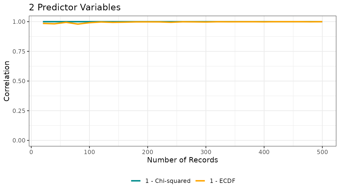

Reproducing the full analysis

The convenience function run_ecdf_mahal_analysis() wraps the original workflow: it runs ecdf_theoretical_niche() for several dimensions (by default 1 to 5) and produces three figures analogous to those in the script.

set.seed(3)
full_res <- run_ecdf_mahal_analysis(dims = 1:5)

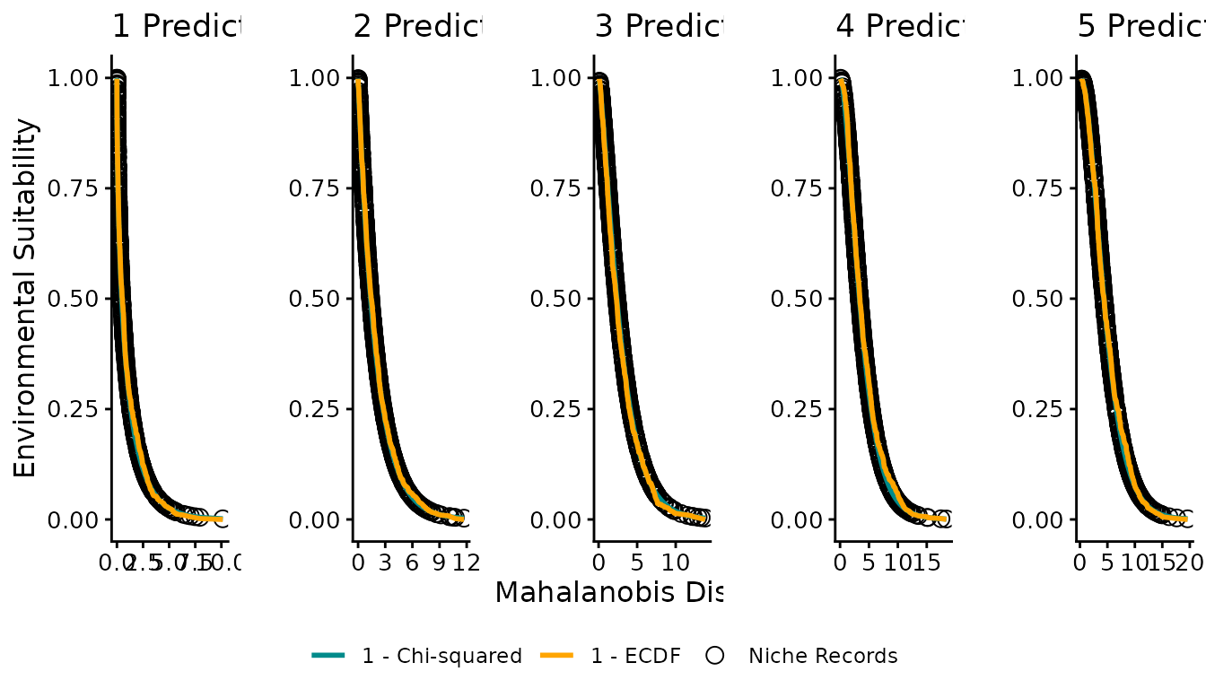
Figure 1: Spatial visualization (2D)

Figure 1 shows the 2D environmental space (two predictor variables) with color representing different suitability definitions: the simulated “true” niche, the chi-squared-based suitability, and the ECDF-based suitability.

full_res$figure1 |> plot()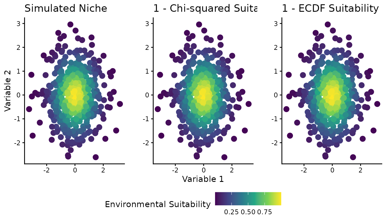

Figure 2: Correlation vs sample size

Figure 2 presents, for each dimensionality, how the correlation between the true niche and each distance-to-suitability transformation changes with sample size.

full_res$figure2 |> plot()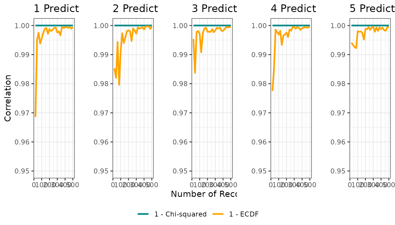

Figure 3: Distance–suitability relationships

Figure 3 plots Mahalanobis distance on the x-axis and suitability on the y-axis, showing how niche records, chi-squared suitability, and ECDF suitability relate across different numbers of predictor variables.

full_res$figure3 |> plot()

Customizing simulations

You can customize key aspects of the simulation by passing arguments to ecdf_theoretical_niche():

res_custom <- ecdf_theoretical_niche(
n = 3,
n_population = 20000,
sample_sizes = seq(50, 1000, 50),
seed = 123
)

res_custom$corplot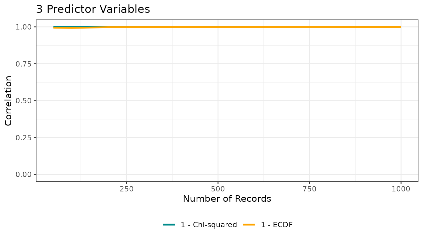

These arguments control the dimensionality, the size of the environmental “background”, and the grid of sample sizes used to compute correlations.

Luíz Fernando Esser