ECDF and Mahalanobis Distance for Empirical Niche Modeling

Luíz Fernando Esser

Introduction

This vignette shows how to use the ECDFniche package to reproduce the simulations from the original manuscript, comparing Mahalanobis distance–based suitability transformations using the chi-squared distribution and the empirical cumulative distribution function (ECDF).

We follow a virtual ecologist approach (Zurell et al. 2010) to evaluate how different transformations of the Mahalanobis distance recover a simulated niche across varying dimensionalities (number of predictor variables) and sample sizes (number of records), and then extend the analysis to a bivariate non-normal environmental space.

library(ECDFniche)
#> Registered S3 methods overwritten by 'ggpp':
#>   method                  from   
#>   heightDetails.titleGrob ggplot2
#>   widthDetails.titleGrob  ggplot2

Multivariate normal niche: ecdf_compare_niche()

In the first set of simulations, we assume that the environmental predictors describing a species’ niche follow a multivariate normal distribution.

Dimensions $p$ range from 1 to 5, and sample sizes $n$ range from 20 to 500 in steps of 20, mimicking increasing numbers of occurrence records.

For each combination of $p$ and $n$, ecdf_compare_niche():

1. Draws a fixed covariance matrix $\Sigma$ by sampling from a Wishart distribution with $p + 2$ degrees of freedom and scale matrix set to zero with a diagonal of 1, ensuring a positive-definite covariance for that $(p, n)$ combination.
2. Generates 30 independent replicates of $n$ records from a $p$-variate normal distribution with mean vector $\mu_p = \mathbf{0}$ (interpreted as the environmental optimum) and covariance matrix $\Sigma$.
3. For each replicate, estimates the sample mean $\mu_r$ and sample covariance $\Sigma_r$ and computes the squared Mahalanobis distance $$D^2 = (x - \mu_r)^\top \Sigma_r^{-1} (x - \mu_r).$$
4. Computes two suitability metrics for every record:

   • Theoretical chi-squared suitability: $$S_{\chi^2} = 1 - F_{\chi^2_p}(D^2),$$ where $F_{\chi^2_p}$ is the cumulative distribution function of the chi-squared distribution with $p$ degrees of freedom.

   • Empirical ECDF-based suitability: $$S_{\text{ECDF}} = 1 - F_{\text{ECDF}}(D^2),$$ where $F_{\text{ECDF}}$ is the empirical cumulative distribution function of the distances.

5. Calculates Pearson’s correlation coefficient between $S_{\chi^2}$ and $S_{\text{ECDF}}$ for each replicate.

This setup mimics a realistic ENM scenario where multivariate means and true covariances are unknown and must be estimated from occurrence records drawn from a correlated environmental space representing the species’ theoretical niche (sensu Hutchinson 1978).

set.seed(1991)
normal_res <- ecdf_compare_niche(
  p_vals = 1:5,
  n_vals = seq(20L, 500L, 20L),
  n_reps = 30L
)

Figure 1: Correlation vs sample size

cor_plot summarizes, for each $p$ and $n$, the mean and standard deviation of the correlation between chi-squared and ECDF suitabilities across the 30 replicates, with individual replicate values shown as grey points. The plot shows the correlation between suitability metrics estimated using the chi-squared and the Empirical Cumulative Distribution Function (ECDF) across sample sizes and numbers of environmental predictors. Each panel shows Pearson correlation coefficients as a function of the number of occurrence records for a given dimensionality p (1 to 5 variables). Correlations are generally very high (rarely < 0.95), increasing with sample size and slightly increasing with dimensionality.

normal_res$cor_plot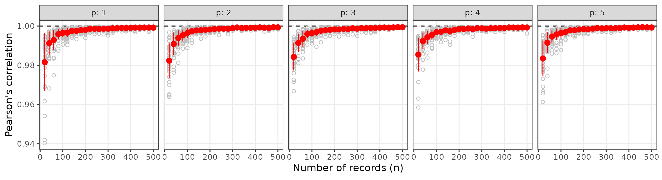

Figure 2: Suitability vs Mahalanobis distance

suit_plot pools observations across sample sizes for each $p$, recomputes an ECDF-based suitability on the combined distances, and compares these to chi-squared curves. The plot shows the relationship between squared Mahalanobis distance (x-axis) and environmental suitability metrics (y-axis) estimated using the chi-squared and the Empirical Cumulative Distribution Function (ECDF) across different numbers of environmental predictors. Grey curves represent the habitat suitability based on the chi-squared distribution while red circles represent habitat suitability via ECDF, highlighting that ECDF closely tracks the theoretical chi‑squared mapping over the distance range.

normal_res$suit_plot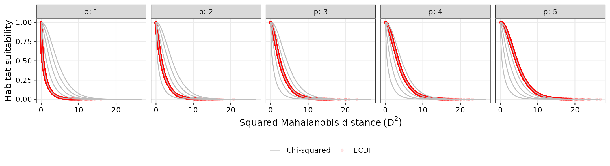

Non-normal bivariate niche: ecdf_nonnormal_niche()

In many real ENM applications, environmental covariates are not jointly normal and species can show complex responses to environmental gradients (Anderson et al. 2022).

To explore this, ecdf_nonnormal_niche() simulates a bivariate environmental space for temperature and precipitation using a Gaussian copula:

• Temperature follows a normal distribution with mean 20 °C and standard deviation 5 °C.
• Precipitation follows a Weibull distribution with shape 2 and scale 10 mm, representing skewed rainfall data.
• The dependence between the two variables is controlled by a correlation parameter $\rho \in \{-0.7, -0.3, 0, 0.3, 0.7\}$, reflecting negative to positive associations observed in climatological studies (e.g. Anderson et al. 2019).

For each $\rho$, the function:

1. Uses a Gaussian copula with correlation $\rho$ to generate a large reference sample of size $N_{\text{ref}}$ (default $10^5$) and derive “true” population mean vector and covariance matrix for the bivariate distribution.
2. For each combination of $\rho$ and sample size $n \in \{20, 50, 100, 200, 500\}$, draws $n_{\text{reps}}$ replicate samples directly from the copula-based bivariate non-normal distribution.
3. Computes squared Mahalanobis distances $D^2$ using the true mean and covariance from the reference sample, isolating the effect of non-normality from parameter estimation error.
4. Calculates:
   • Chi-squared suitability $S_{\chi^2} = 1 - F_{\chi^2_2}(D^2)$, which is theoretically “wrong” under non-normality but serves as the standard parametric benchmark.
   • ECDF-based suitability $S_{\text{ECDF}} = 1 - F_{\text{ECDF}}(D^2)$.
5. Returns per-replicate correlations and observation-level data, plus a summary plot comparing the two suitabilities.

set.seed(1991)
nonnormal_res <- ecdf_nonnormal_niche(
  rho_vals = c(-0.7, -0.3, 0, 0.3, 0.7),
  n_vals   = c(20L, 50L, 100L, 200L, 500L),
  n_reps   = 10L,
  N_ref    = 1e5,
  temp_function = "qnorm",
  temp_parameters = list(mean = 20, sd = 5),
  prec_function = "qweibull",
  prec_parameters = list(shape = 2, scale = 10)
)

Figure 3: Suitability vs distance under non-normality

suit_plot shows ECDF-based suitability (colored by $\rho$) and chi-squared suitability (red points) as functions of $D^2$, faceted by sample size. Plots highlight the sensitivity of chi-squared and ECDF suitability metrics to sample size and variable correlation in non-normal bivariate data. Internal histograms represent the distribution of ECDF-based values around the chi-squared-based suitability. The ECDF estimator shows higher stochasticity in small samples but converges to the chi-squared expectation in larger samples.

nonnormal_res$suit_plot
#> Warning: Removed 2 rows containing missing values or values outside the scale range
#> (`geom_bar()`).
#> Removed 2 rows containing missing values or values outside the scale range
#> (`geom_bar()`).
#> Removed 2 rows containing missing values or values outside the scale range
#> (`geom_bar()`).
#> Removed 2 rows containing missing values or values outside the scale range
#> (`geom_bar()`).
#> Removed 2 rows containing missing values or values outside the scale range
#> (`geom_bar()`).

Customizing simulations

You can customize key aspects of both simulations to reproduce or extend the analyses:

• Multivariate normal niche (ecdf_compare_niche()):
  • p_vals: set of dimensions (e.g. 1:10) to evaluate high-dimensional behavior.
  • n_vals: sample size grid, e.g. smaller n to explore the effect of limited records.
  • n_reps: number of replicates per combination for more stable summaries.

res_custom_normal <- ecdf_compare_niche(
  p_vals = 2:4,
  n_vals = seq(20L, 200L, 20L),
  n_reps = 50L,
  seed   = 42
)
res_custom_normal$cor_plot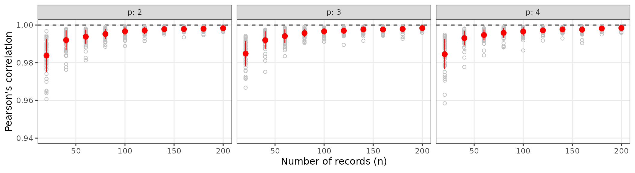

• Non-normal bivariate niche (ecdf_nonnormal_niche()):
  • rho_vals: alternative dependence structures.
  • n_vals, n_reps: sample size and replication design.
  • N_ref: reference population size; larger values approximate the true parameters more closely.

res_custom_nonnorm <- ecdf_nonnormal_niche(
  rho_vals = c(-0.5, 0, 0.5),
  n_vals   = c(30L, 100L, 300L),
  n_reps   = 20L,
  N_ref    = 5e4,
  temp_function = "qnorm",
  temp_parameters = list(mean = 20, sd = 5),
  prec_function = "qweibull",
  prec_parameters = list(shape = 2, scale = 10),
  seed     = 123
)
res_custom_nonnorm$suit_plot
#> Warning: Removed 7 rows containing non-finite outside the scale range
#> (`stat_bin()`).
#> Warning: Removed 2 rows containing missing values or values outside the scale range
#> (`geom_bar()`).
#> Removed 2 rows containing missing values or values outside the scale range
#> (`geom_bar()`).
#> Removed 2 rows containing missing values or values outside the scale range
#> (`geom_bar()`).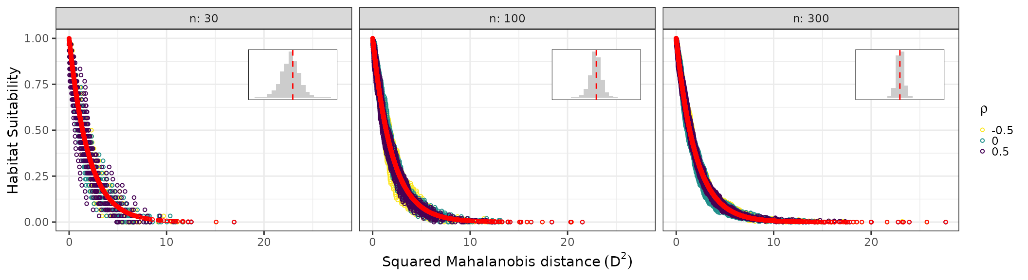

Together, these simulations illustrate when the traditional chi-squared transformation is reliable and when the ECDF-based approach provides a more robust mapping from niche-based distances to habitat suitability, particularly when environmental covariates deviate from multivariate normality.