Obtain the Partial Dependence Plots (PDP) to each variable.
Usage
pdp_sdm(i, spp = NULL, algo = NULL, variables_selected = NULL, mean.only = FALSE)

get_pdp_sdm(i, spp = NULL, algo = NULL, variables_selected = NULL)
Arguments
- i
A
input_sdmobject.- spp
A
charactervector with species names to obtain the PDPs. IfNULL(standard), the first species inspecies_names(i)is used.- algo
A
charactercontaining the algorithm to obtain the PDP. IfNULL(standard) all algorithms are mixed.- variables_selected
A
character. If there is a subset of predictors that should be ploted in this, it can be informed using this parameter.- mean.only
Boolean. Should only the mean curve be plotted or a curve to each run should be included? Standard is FALSE.
Examples
# Create sdm_area object:
sa <- sdm_area(parana, cell_size = 100000, output_crs = 6933)
#> ! Making grid over study area is an expensive task. Please, be patient!
#> ℹ Using GDAL to make the grid and resample the variables.
# Include predictors:
sa <- add_predictors(sa, bioc) |> select_predictors(c("bio1", "bio12"))
#> ! Making grid over the study area is an expensive task. Please, be patient!
#> ℹ Using GDAL to make the grid and resample the variables.
# Include scenarios:
sa <- add_scenarios(sa)
# Create occurrences:
oc <- occurrences_sdm(occ, occ_crs = 6933)
# Create input_sdm:
i <- input_sdm(oc, sa)
# Pseudoabsence generation:
i <- pseudoabsences(i, method = "random", n_set = 3)
# Custom trainControl:
ctrl_sdm <- caret::trainControl(
method = "repeatedcv",
number = 2,
repeats = 1,
classProbs = TRUE,
returnResamp = "all",
summaryFunction = summary_sdm,
savePredictions = "all"
)
# Train models:
i <- train_sdm(i, algo = c("naive_bayes"), ctrl = ctrl_sdm)
#> Loading required package: ggplot2
#> Loading required package: lattice
# PDP plots:
pdp_sdm(i)
#> `geom_smooth()` using method = 'loess' and formula = 'y ~ x'
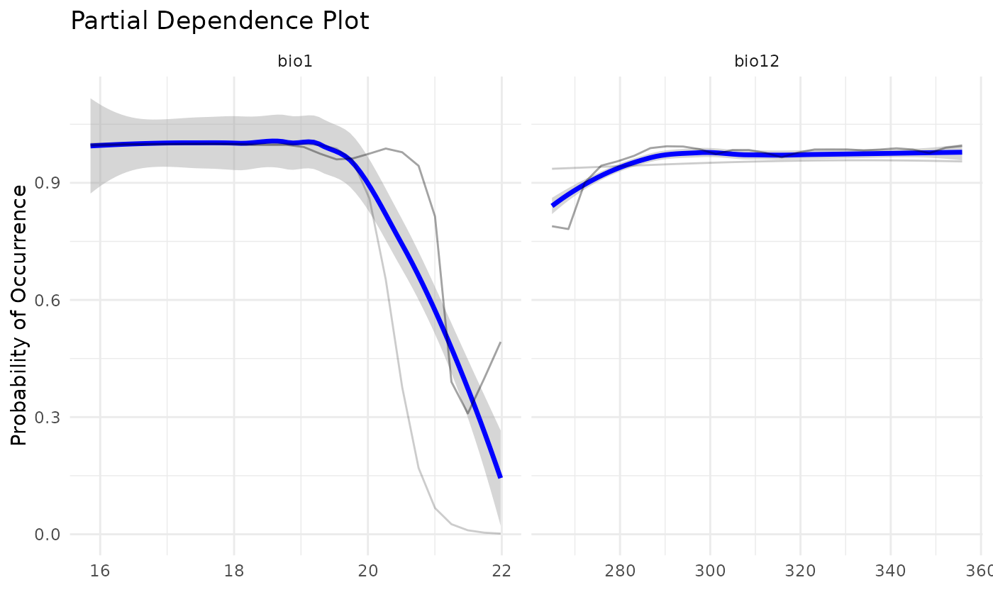 get_pdp_sdm(i)
#> $naive_bayes
#> # A tibble: 129 × 4
#> id yhat variable value
#> <chr> <dbl> <chr> <dbl>
#> 1 naive_bayes_pa1 0.987 bio1 16.6
#> 2 naive_bayes_pa1 0.986 bio1 16.9
#> 3 naive_bayes_pa1 0.984 bio1 17.1
#> 4 naive_bayes_pa1 0.982 bio1 17.4
#> 5 naive_bayes_pa1 0.979 bio1 17.6
#> 6 naive_bayes_pa1 0.976 bio1 17.9
#> 7 naive_bayes_pa1 0.971 bio1 18.1
#> 8 naive_bayes_pa1 0.965 bio1 18.4
#> 9 naive_bayes_pa1 0.958 bio1 18.6
#> 10 naive_bayes_pa1 0.949 bio1 18.9
#> # ℹ 119 more rows
#>
get_pdp_sdm(i)
#> $naive_bayes
#> # A tibble: 129 × 4
#> id yhat variable value
#> <chr> <dbl> <chr> <dbl>
#> 1 naive_bayes_pa1 0.987 bio1 16.6
#> 2 naive_bayes_pa1 0.986 bio1 16.9
#> 3 naive_bayes_pa1 0.984 bio1 17.1
#> 4 naive_bayes_pa1 0.982 bio1 17.4
#> 5 naive_bayes_pa1 0.979 bio1 17.6
#> 6 naive_bayes_pa1 0.976 bio1 17.9
#> 7 naive_bayes_pa1 0.971 bio1 18.1
#> 8 naive_bayes_pa1 0.965 bio1 18.4
#> 9 naive_bayes_pa1 0.958 bio1 18.6
#> 10 naive_bayes_pa1 0.949 bio1 18.9
#> # ℹ 119 more rows
#>